
|
|
CCALMR EBS OGI OHSU |
ACE/gredit is started by typing one of the following commands:
xmgredit -f [grid file]The first command assumes that a grid file already exists, and that it will be initially loaded as both the background grid and the edit grid for the session of ACE/gredit initiated with the command. The flag -f is optional, referring to the format of the grid file (-f for binary, blank for ASCII).xmgredit -m [minimum distance] -b [bathymetry file] -w
xmgredit -m [minimum distance] -b [bathymetry file] -f [grid file]
xmgredit -W [xmin ymin xmax ymax]
The second command assumes that the user wants to generate the background grid from a set of unstructured data points, each with an assigned depth, and that no edit grid is previously available. The meanings of the flags and read-in parameters are as follows:
-m [minimum distance]
Sets the minimum distance allowed between nodes when triangulating a file of bathymetry. The ensemble of build points is tested for the minimum distance criterion, and points not satisfying the criterion are eliminated from the triangulation process. The -m flag is optional (but highly recommended); if used, it requires the use of the -b flag described below. The [minimum distance parameter] is an user-specified real number, in units consistent with those of the bathymetry file.
-b [bathymetry]
The flag -b indicates that the background grid will be build by triangulation from a set of unstructured points, contained in a bathymetry file. The parameter [bathymetry] is the user-specified name of this file.
-w
Generates a two-element editable grid, based on the geometric limits found in the file of bathymetry.
The third command is a combination of the first and second ones. It assumes that the background grid will be generated from a bathymetry file, but that an edit grid file is already available. All flags and parameters have already been described.
The fourth command generates a 2-triangle grid between the specified coordinates, with uniform depth of 1m.
Typing
xmgredit [return]
will bring a help text, describing the different options described above. The ACE/gredit code will not be activated.
Typing
xmgredit -v [return]
will in addition indicate the date of the compilation of the current version of ACE/gredit..
The formats of all files introduced above, and others used by ACE/gredit are listed in Chapter 3.
The initial user interface to ACE/gredit consists of the menu bar on the top, a drawing area, a toolbar on the left, and a status line on the bottom of the display. Using pulldown menus, the menu bar allows access to a variety of features used to create, modify, and report on the status of grids.

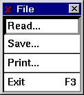
The pulldown menu File controls the reading/writing of data files (through two separate popups), printing of the drawing area, and allowing the user to exit ACE/gredit.

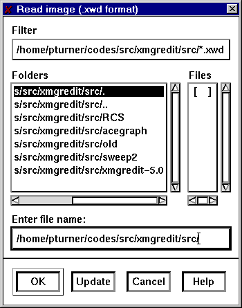
Use the Filter selection to get a listing of files in the directory.
Select the type of file using the selection Read object. The choices are:
Use the Selection item to enter the specific file name.
Click on the OK button to read the desired ACE/gredit object. On success the drawing area is refreshed, and the new object (if drawable) is drawn.
Similarly, selecting the Save popup

opens a dialogue allowing data to be written to disk.
Select the object to write, the file format, and the name of the file and click on Accept.
To generate a hardcopy, select the Print item from the File menu.

Select the device, either PostScript landscape, PostScript portrait, FrameMake .mif landscape, or FrameMaker .mif portrait.
Print control string: The meaning of this item depends on the selection chosen in the Print to: item above. If the printing is to be done to a printer, enter the string used to spool. If printing is to be done to a file, enter the file name.
Press Accept to register the changes, Print to print the current display, or Cancel to close the popup without printing. The Accept button does not print.
Selecting Exit terminates ACE/gredit, upon the user's acceptance of a confirmation question. Note that all data that was not previously saved to disk will be lost upon the termination of ACE/gredit.
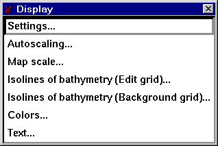
Items in the Display pulldown menu affect how and which objects are drawn on the drawing area.
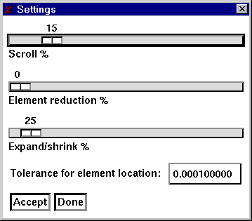
Scroll % sets the amount of movement for the arrow buttons located on the main panel. With the mouse, press on the hilighted bar while holding the mouse button down and move to the right (increasing scroll) or left (decreasing scroll). Changes in the position take effect immediately and affect the next and subsequent presses of the scrolling arrows on the main panel.
Element reduction % sets the amount to shrink elements about their centers. This is sometimes convenient to check whether elements exist and/or are properly formed. Changes in this item take effect the next time the grid is re-drawn.
Expand/shrink % sets the amount to expand or shrink the grid when the Z or z buttons are pressed, respectively.
Tolerance for element location sets the value to use to determine if a point is in an element.
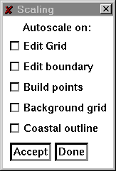
Autoscale the display with regard to one or more features
:
Select the object(s) to use to set the scale, then click on Accept. The display will be scaled in such a manner that the selected object(s) will be contained in the display.
Set the

Set the map scale legend by selecting the length of the legend, the units of the legend, and
other properties. Use
Limits (status only): Display the minimum and maximum values of the depths in the edit
grid.
Draw isolines: Select the method used to draw isolines. There are three selections,
Lines, Filled, or Both. If Lines is selected, isolines are drawn as lines at the isoline
values. Filled draws filled contours with the isoline values representing lower bounds.
With Both, isolines are draw as lines and color filled contours. Use View/Colors to set
the colors for filled contours.
Precision: Set the number of places to the right of the decimal point for labels in
the legends and in the assignment of the isoline values.
# of isolines: Set the number of isolines to use for both the start/step or specified
spacing of isolines.
Isoline spacing by: A choice item, either Start/step or Specified. If Start/step is selected, the the values for Start and Step below are used to determine the spacing of isolines.
Start value: In the Start/step method of isolines spacing, the starting value for isolines.
Step value: In the Start/step method of islolines spacing, the increment between successive isolines.
Precision: Number of decimal places to the right of the decimal point to use for the isoline levels.
The two columns of text items occupying the center of this popup are used for the Specified method of isoline spacing and to display the values computed by the selection of the Start step method.
Click on Accept to register the changes. Autoscale will update the values
in the Limits text item.
Set isolines of bathymetry (background grid)
This popup is identical to the previous popup, but operates on the background grid only.
Set the scaling of the drawing area
Set the viewport or clipping region of the drawing area
ACE/gredit uses 48 colors divided into three sections, one reserved for annotation,
the second is used for isolines of bathymetry, the third for isolines of concentrations
and elevations. Each sections contains 16 colors for a total of 48.
Each color may be individually set, or linearly interpolated using either the RGB color
model (red, green, blue) or the HSV color model (hue, saturation, and value).
RGB values range from 0 to 255 for each of the three primary colors. A value of 0 for any
primary color means that this component is not included in creation of the selected
color. Black is the color composed of RGB values (0, 0, 0), or no contribution from any
of the three primary colors. White is formed when each of the primary color values are
255. To form the most solid blue, set the RGB values to (0, 0, 255).
Colors are set using the HSV color model by selecting a hue, or color, then varying the
amounts of white (saturation), and black (value). The hue is a value from 0 to 360, and
is measured in degrees around a color wheel that begins with red (hue = 0), and cycles
through the colors, winding up at red again (hue = 360). Going from 0 to 360 degrees, a
color goes from red, to yellow, to green, to cyan, to blue, to violet, then back to red at
360. The saturation of a color is a measure, from (0, 1.0), of the amount of the color to
add. A saturation value of 0.0 will be white regardless of the hue, as this means that none
of the hue will be used to form the color. A completely saturated color, i.e. a saturation
value of 1.0, indicates that there is no white in this color. The value quantity measures
the how light the color determined by the hue and saturation values will be. A value of 0
means that the color will appear black, a value of 1 indicates that the color will be the
maximum brightness allowed by the hue and saturation values.
To set a particular color, click on the color then adjust the sliders provided in either
the RGB or HSV color spaces. As there is a mapping to and from each color space,
changing a value in one color space will cause a corresponding change in the other.
To set a range of values, use linear interpolation. Select the color space in which to
do the interpolation, the starting color and ending color, then click on Interpolate
to perform a linear interpolation from the starting to the ending color. The starting
and ending colors are not affected by the interpolation, it applys to the intervening
colors only.
Use Undo to reverse the effects of Interpolate. Use Reset to set the colors to the start-up values. Read and Write bring up popups that allow the current colormaps to be read or written to disk. Use Done to close the popup.
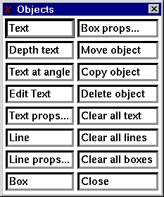
Use this popup to place annotative text, lines, and rectangles on the drawing area.
Text: To draw a text string, click on Text, then click at the location on the drawing area to place the text and type the text directly onto the drawing area.
Text at angle: With two successive mouse clicks on the drawing area, define a line to specify the angle at which the text is to be drawn, then click again at the location of the start of the text line and type in the desired text.
Edit Text: Selecting this item and click near the start of the text line to edit.
Text props: Set the color, line width, rotaion, and justification of text. This popup only affects strings created after using this popup.
Line: Click at the start and end of the line.
Line props: Set the color, line width, line style, and arrows of lines created after the use of this popup.
Box: Create a rectangle by clicking on opposite corners of the rectangle.
Box props: Set the color, line width, line style, and fill style of rectangles created after the use of this popup.
Use Move, Copy, and Delete to manipulate existing objects.
Use Clear all text, Clear all lines, and Clear all boxes to remove each of these types of objects.
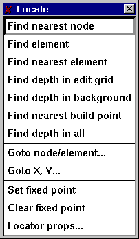
Displays information concerning individual nodes and elements, and places the
pointer at user-selected nodes and elements.
Display information about the node nearest the pointer when the left mouse button is pressed. The node number, the location and the depth at this node are displayed in the Locate message item on the main panel.
Display information about the element containing the pointer when the left mouse button is pressed.
Display information about the element nearest the pointer when the left mouse button is pressed. The element number, the numbers of nodes defining this element, the area, and the equivalent radius and the depth at this node are displayed in the Locate message item on the main panel.
Clicking at a point in an element of the edit grid containing the pointer displays the interpolated depth at that point in the Locate message item on the main panel..
Clicking at a point in an element of the background grid containing the pointer displays the interpolated depth at that point in the Locate message item on the main panel.
Display the location and depth of the build point nearest the pointer when the left mouse button is pressed.
Report on the depth in both the edit and background grids when the left mouse button is pressed.
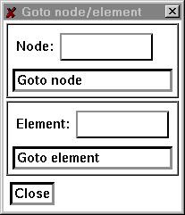
Warp the cursor to a user specified node or element.
Selecting the Goto node/element item brings up a popup allowing a node or element number to be entered. pressing the Goto node or Goto element button moves the pointer to that node or element.
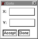
Use Goto X, Y to warp the pointer to a particular location in the drawing area.
Set the point to use as a fixed point from which positions are computed for the locator message item.
Disable the use of a fixed point for the locator position.
Set the format and precision to use for the display of the pointer position.
Locator: Toggle the continuous display of the pointer position. When ON, the pointers posistion is displayed continuously in the locator item on the main panel, when OFF, the position of the pointer is displayed only when the left mouse button is pressed.
Locator display type: Set the transformation used to compute the locator's position. There 6 choices
X, Y: Display the pointer location in terms of the doamin coordinate system.
DX, DY: If the locator fixed point is set, display the location of the pointer
as the difference between the pointer's location in the grid coordiante system and
the fixed point. If no fixed point is set, then the display is the same as for [X, Y].
Distance: If the locator fixed point is set, display the difference in distance
between the pointer's position in the grid coordinate system and the fixed point. If
no fixed point is set, then display the distance from the origin.
R, Theta: If the locator fixed point is set, display the position of the pointer
in polar coordinates relative to the fixed point. If no fixed point is set, display
the position of the pointer in polar coordinates relative to the origin.
VX, VY: Display the pointer's position in viewport coordinates.
SX, SY: Display the pointers posistion in screen coordinates.
The items Format X and Format Y select the format of the numerical display
of the pointer position. Either General, Decimal, or Exponential. General selects one of
decimal or scientific notation to display the location, depending on the magnitude of
the numbers. Decimal selects a fixed number of significant digits, exponential uses
scientific notation for the display.
The number of places to the right of the decimal point is set using the
Precision X and Precision Y items.
Explicitly set the fixed point position using the Fixed point X and
Fixed point Y text items.
Toggle the use of the fixed point using the Fixed point choice item. Selecting ON
will cause the locator display to use the fixed point in computing the pointer
location if the locator display type is [DX, DY], [DISTANCE], or [R, Theta].
Press Accept to register the changes, Reset to restore the default values,
and Done to close the popup.
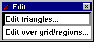
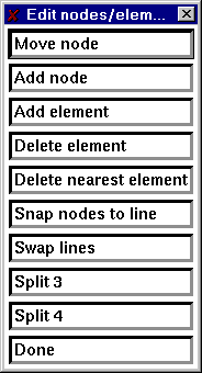
Call the pop-ups that control the editing of nodes, elements and associated features, either in an individual basis, over the entire grid, or within selected regions.
Individual operations
For grids composed strictly of triangles, the following operations may be performed
on nodes and elements of the grid.
The move node item allows the location of individual nodes to be changed by using the
mouse.
Select the Move node item and click near the node to be moved and click again with
the pointer at the new location.
The coordinates in the table of nodes defining the locations will be updated to
reflect the new location for each node that is moved. This procedure may be repeated
as often as desired, as once the Move node item is selected, the mouse will stay in
this mode until the right mouse button is pressed or another action item is selected.
The add node item allows a node to be added to the table of nodes. Select the Add node
item and click at the location of the new node, the coordinates of the new node will be
appended to the table of nodes. Adding nodes may be repeated as often as desired until
the right mouse button is pressed or another action item is selected.
Note:
Merely adding nodes to the table of nodes does not automatically create new elements. To
use the add node function effectively, it should be used with the Add element
function described below.
Add an element to the table of elements in the editable grid.
Click on three nodes in a counter-clockwise fashion to specify the nodes for the new
element. If additional elements are required, repeat as needed as this function
repeats until the right mouse button is pressed. The new element is added to the
table of elements.
Remove elements from the table of elements.
Click on the Delete element button. Click in the interior of the element to be removed.
Repeat as needed, when completed, use the the middle mouse button to register the
deletions. To cancel, press the right mouse button. Elements are removed from the
table of elements.
Remove the element nearest the pointer from the table of elements.
Click near the element to be removed. Repeat as needed, when done, use the the middle
mouse button to register the deletions. To cancel, press the right mouse button. Elements
are removed from the table of elements.
Note:
Delete nearest element uses the centers of elements to determine which element is nearest the pointer.
Move selected nodes so that they lie on a previously defined line.
Snapping nodes require the definition of a line. After selecting the snap to line
option, click at the beginning of the line, and again at the end of the line. Click on
each node to be snapped, when done, press the middle mouse button to register the
collection of nodes to be snapped. The right mouse button cancels the operation.
Result
Each selected node is translated to the line by computing the shortest distance from the node to the line.
Swap the shared lines between elements.
Select the two elements with a shared edge by clicking on each element.
Split an element into three elements.
Click in the interior of the element to be split, repeat as needed. When done, use the the middle mouse button to split each selected element into 3 elements. To cancel, press the right mouse button.
Result
Elements are split into 3 by joining the vertices of each selected element with the center of the element.
Note
Generally, the elements formed by this procedure are poorly formed. Triangulating will rearrange the elements in a more acceptable configuration.
Split an element into four elements.
Click in the interior of the element to be split, repeat as needed. When completed, use
the the middle mouse button to split each selected element into 4. To cancel, press
the right mouse button.
Result
Elements are split into 4 elements using a division based on joining the midpoints of
the element edges.
Note
This function forms elements that may not be properly formed. Specifically, nodes are created that are not necessarily shared by adjacent elements. Triangulating will rearrange the elements to a more acceptable configuration.
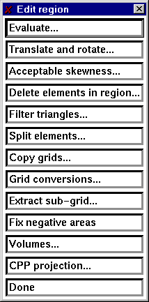
Operations over an entire grid or in specified regions
The popup for operations within specified regions includes several items.
Evaluate a mathematical expression on the co-ordinates or depths of nodes. Variables are x, y for the coordinate directions and depth for the depth at a node.
Allows the translation and rotation of a grid
Enter values for the translation, the rotation (in degrees), and the point about which to rotate, then click on Accept.
Note: The order of operations is translation followed by rotation.
During the process of grid creation, occasional skinny elements are formed. Selecting this item marks these elements and optionally allows them to be deleted.
Remove all elements inside or outside the current region.
Split elements into 3 or 4 elements inside or outside the currently defined region.
Select the grid to copy from and the grid to copy to. There are 5 slots for grids in ACE/gredit plus one for the background grid.
Select the number of the grid that will hold the extracted sub-grid, then click on Apply. With successive mouse clicks, form a region containing the sub-grid. Press the middle mouse button to select all elements in the region to use to form the new grid. To make this grid active, copy it to grid 0 (unless grid 0 was selected as the destination for the sub-grid).
Perform a check on each element to make sure that each is formed in a counter-clockwise fashion.
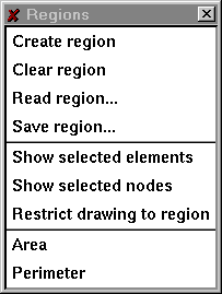
Select a polygonal region used to restrict operations to a particular segment of the editable grid. Successive clicks at the vertices of the polygon, builds the region. Use the middle mouse button to register the defined polygon, or the right mouse button to cancel.
Remove the currently defined region, if any.
Compute the area of a polygonal region.
Compute the perimeter of a polygonal region
This menu allows the creation and edition of edit internal and external
boundaries.
Individual items in the menu are discussed below.
Define the outer boundary of the editable grid. Define a boundary by clicking with
the left mouse button at the locations of the boundary in a counter-clockwise fashion.
Change the location of one or more external boundary points.
With the left mouse button click near the node to be moved, then click again
at the new location.
Add a point to an existing boundary.
Click on the nodes to either side of the location of the new boundary node, then click
at the location of the new boundary node.
Define a boundary in the interior of the editable grid. Define a boundary by clicking
with the left mouse button at the locations of the boundary in a clockwise fashion.
Change the location of one or more internal boundary points. With the left mouse button
click near the node to be moved, then click again at the new location.
Remove an internal boundary by clicking near the boundary point with the left mouse button.
Determine, from the elements defining the editable grid, the external boundary and all interior boundaries.
Remove the definition for the external boundary.
Remove all interior boundaries.
Display the boundary as a line.
Display the boundary using markers at each node.
Display the boundary as node numbers.
This menu controls the placement of build points and their triangulation into a properly
formed finite element grid.
Define build points using the mouse. With the left mouse button, click at the
location in the domain to place the build point.
Click near a build point to remove the build point from the collection of build points.
Select a build point by clicking near the point then move the mouse to the new location of the build point. Click again to place the point.
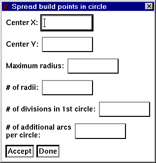
Create build points according to a circular pattern.
In the items Center X and Center Y enter the point to use as the center of the circle. Enter the maximum radius in the text item labeled Maximum radius. The item # of radii gives the number of divisions that will be made from the maximum radius. The next two items determine the density of points as the radii increases.
Create build points within a rectangular region, according to a either regular (rectangular or rectangular offset) or random patterns
.
Create build points according to one of four pre-specified criterion. The Courant number and maximum dimensionless criteria are currently set for flow models (i.e., rely on a depth-related celerity, c=sqrt(gh)).
The minimal requirements for automatic generation of build points, are an edit grid boundary and a background grid of bathymetry. If the boundary is to be created, then a coastal outline needs to be present also.
For build point generation, a rectangular grid (referred to here as the auxillary grid) is
created, such that the bounding rectangle of the background grid is covered. The resolution
of this auxilary grid is set by the numeric text item labelled Grid delta. To change
the limits of the auxillary grid use the Xmin, Xmax, Ymin, Ymax items. The algorithm
starts by interpolating the depth from the background grid to the vertices of the auxillary
grid. Build points are formed by searching for the vertex in the auxillary grid with the
greatest depth, then spiraling out from this vertex accumulating the depth and locations of
unvisited vertices. The accumulated depths are used to compute the value of the test criteria
and compared with the limiting value (either the minimum allowable dimensionless wavelength
or Courant criteria). When the criteria is met, a build point is placed at the average location
of the vertices visted. If the number of loops performed in the process of spiralling out from
the center vertex is greater than the amount specified in the numeric text item,
Maximum loop, the search is halted and a build point placed at the average location.
The item Create boundary toggles the automatic generation of the edit grid boundary.
Because it is unlikely that the coastal outline and the background bathymetry will match in
every case along the boundary, it is necessary to establish a minimum value for the depth at
the boundary using the numeric text item Minimum depth at boundary.
Use the item Minimum depth in domain to set a minimum allowable depth in the interior
of the edit grid boundary. This is necessary as the numerical criteria used to place build
points will fail in the presence of negative depths.
Make the nodes of the editable grid the current set of build points.
Add the nodal positions in the editable grid to the currently defined set of build points.
Add the positions of the centers of all elements to the current set of build points.
Add the positions of the boundary to the current set of build points.
Perform a Delauney triangulation on the current set of build points, removing all elements that are formed outside the external boundary or inside internal boundaries providing said boundaries exist.
Define the distance treshold below which two build points are collapsed into a single point.
Re-shapes existing elements, to create triangles that are more equilateral in shape. More than one application may be necessary.
Toggle drawing of build points
This menu allows the execution of some final-stage, model-oriented operations. These
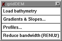
operations are currently limited to the loading of the bathymetry to the edit grid nodes,
and to the generation/display of bathymetric profiles. This is a menu in expansion
phase.
Using the background grid, interpolate depths for the nodes in the editable grid.
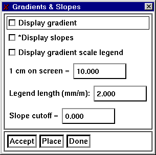
Use this feature to display the gradients and slopes of the bathymetry.
Take a one-dimensional `slice' through the editable and/or background grid, for which the bathymetry profile can be examined.
Minimize the bandwidth of a grid of linear triangles.
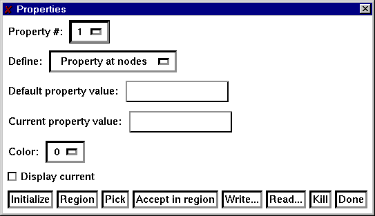
Use the properties popup to define quantities or groups of elements.
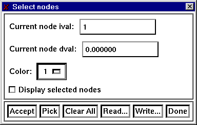
Select the number of the property to define. Use the item Define to select if the property is to be defined at the nodes of the grid, or at the elements. The Default property value is used to assign a value to all nodes (elements) for initialization. The Current property value is the selection that will be used in the Pick and Region operations described below. Set the color for the current property and toggle the display of the current values.
Click on Initialize to set the properties to the default value defined above. Use Region to define a polygonal region containing nodes (elements) that will be assigned the value of the Current property value. Use Pick to select individual nodes (elements). Accept region sets the property values of all nodes (elements) that are presently contained in the Region. Use Write to write the current state of the property values and Read to read in previously defined values.
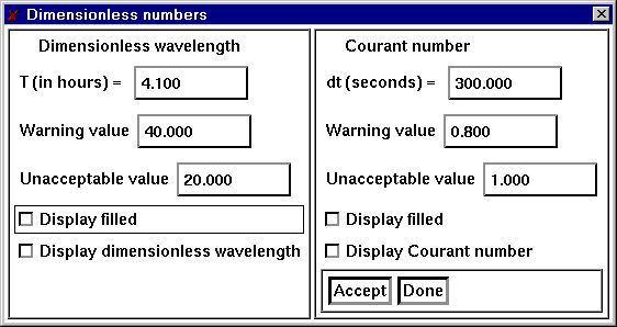
Use the functions provided here to determine if the current grid satisfies specific numerical criteria. At present there are two selections that may be displayed simultaneously.
The dimensionless wavelength, Lm, is defined by:
sqrt(g*h)*T/delX
The Courant number, Cu, is defined by:
sqrt(g*h)*delT/delX
Report on items pertaining to the edit grid, build points, and boundaries.
Set isolines of bathymetry (edit grid)

Viewport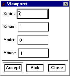
Read an image to display on the drawing area.
Set colors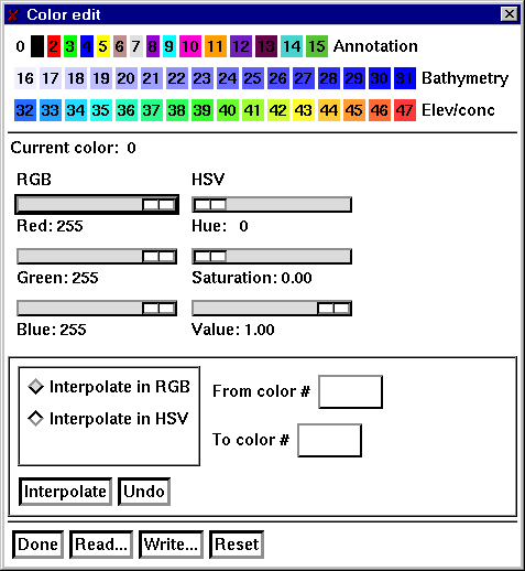

Regions
Boundaries

Build


gridDEM
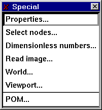
Application specific popups.
Last Modified: January 19, 1997
Copyright © 1999 Center for Coastal and Land-Margin Research