Coupling with NWM

Overview

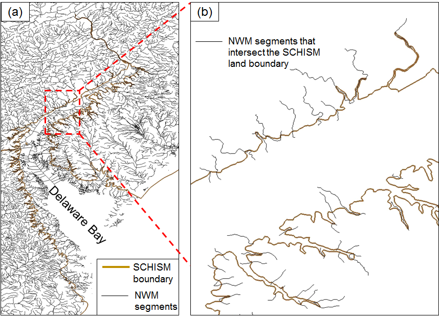
The streamflows from the NWM v2.0 reanalysis database are injected into the SCHISM domain as point sources/sinks at the intersections between NWM segments and SCHISM land boundaries:

NWM data preparation

Following the instructions of the complete archive of NWM data version 2.0, the NWM outputs can be downloaded by "aws" or "python -m awscli". For example, to download the data of June, 2018:


   	  aws s3 cp s3://noaa-nwm-retro-v2.0-pds/full_physics/2018/  . --no-sign-req --recursive --exclude "*" --include "201806*CHR*"

The downloaded data look like:


		...
		201806301400.CHRTOUT_DOMAIN1.comp
		201806301500.CHRTOUT_DOMAIN1.comp
		201806301600.CHRTOUT_DOMAIN1.comp
		201806301700.CHRTOUT_DOMAIN1.comp
		201806301800.CHRTOUT_DOMAIN1.comp
		...

The data should cover your run period (preferrably having a few days past the end date of your run). You'll need to provide the path to your NWM data folder in the next step.

Scripts

In the ECGC (East Coast and Gulf Coast) setup, the Matlab scripts used in the Delaware Bay setup have been replaced by a more efficient Fortran script, written by Dr. Wei Huang (whuang@vims.edu). The first step is finding the intersections between NWM segments and SCHISM land boundaries and generating sources/sinks. The script is:


      [SCHISM_Git_dir]/schism/src/Utility/Pre-Processing/NWM/NWM_coupling/coupling_nwm.f90

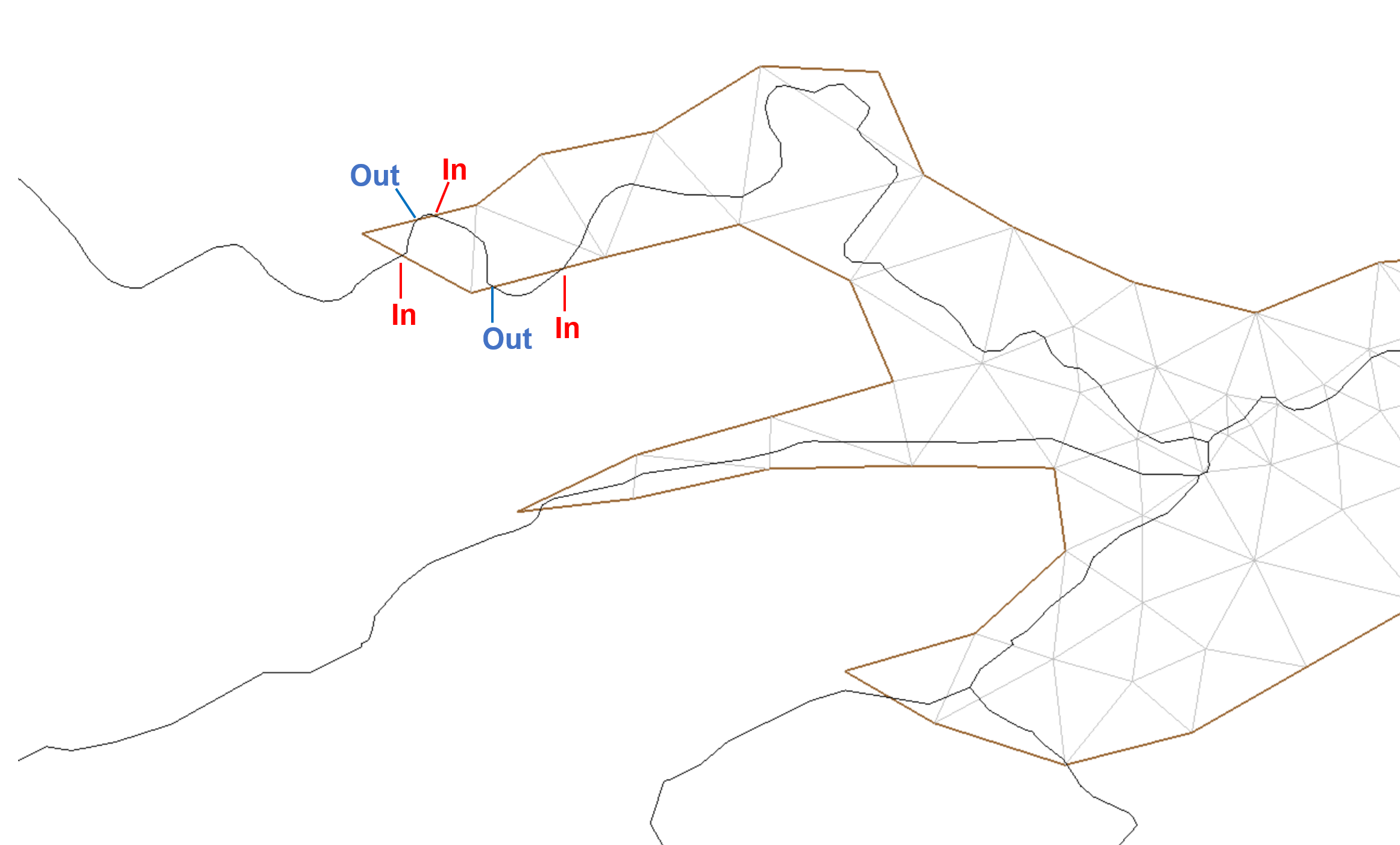
An additional step in the new setup is combining sources and sinks within a specified radius. When an NWM segment is not well aligned with the SCHISM land boundary, it can go in and out of the model domain frequently within a short distance. In this case, it is preferrable to simplify the distribution of sources/sinks. In practice, we merge each sink into its neighboring (within 4 km) sources if there are any. This is done by


			[SCHISM_Git_dir]/schism/src/Utility/Pre-Processing/NWM/NWM_coupling/combine_sink_source.F90

The manual steps are described in:


			[SCHISM_Git_dir]/schism/src/Utility/Pre-Processing/NWM/NWM_coupling/README

Alternatively, you can "cp -rL" the NWM_coupling/ folder to your run directory, "cd $your_run_dir/NWM_coupling/", then do "./auto.pl"

The following files will be generated and copied to your run directory:

source_sink.in: element IDs where sources and sinks are imposed.
vsource.th: time (seconds; first column) history of flow rate (m³/s; the 2nd to the last columns) at each source (inflow) element.
msource.th: time (seconds; first column) history of tracer concentrations at each source element.
vsink.th: time (seconds; first column) history of flow rate (m³/s; the 2nd to the last columns) at each sink (outflow) element.

After the source/sink files are generated, it is recommended to visualize them and make sure nothing is obviously wrong. You can use the "viz_source.m" (depending on "load_hgrid.m") under "NWM_coupling/" for visualization.

For example, the plot below illustrates the magnitudes of point sources (time-averaged) by circles of different sizes:

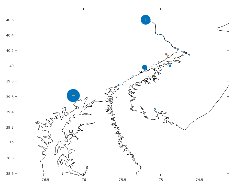
In this case, the largest source inside the Delaware Bay is flowing into the Delaware River and the second largest is into the Schuylkill River.

Note: the procedures below are only for the Delaware Bay setup, which are not needed unless you want to exactly reproduce the Delaware Bay model inputs. The Fortran scripts above are recommended for all later setups.

Defining the portion of SCHISM boundary to be coupled

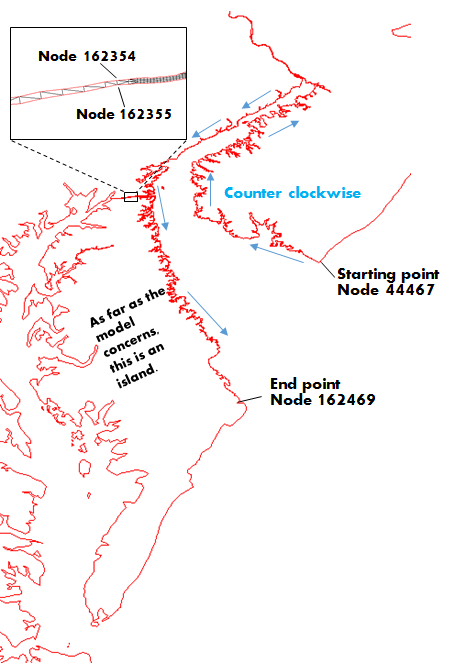
In most cases, this should be as straightforward as picking the starting point (Node 44467 in the figure below) and the end point (Node 162469). The model coupling script will extract the portion of the SCHISM boundary from the starting point to the end point in a counter-clockwise fashion. However, the current setup is a little trickier: there are two SCHISM boundaries involved here due to the existence of the DB-CB channel. As a result, two more points are needed to specify the location where you want to cross the DB-CB channel (zoomed-in view in the figure below).

Generating source/sink input files

A group of Matlab scripts and the shapefile of NWM v1.2 are provided under this folder (NWM_Coupling_Old_Matlab/) for automatically generating the files specifying point sources/sinks:

!! Important !!: if you are using a different hgrid.ll from the sample grid under "NWM_Coupling_Old_Matlab", you need to also remove *.mat and X_NWM_SEG* under "NWM_Coupling_Old_Matlab". These files are generated at the first run to save time for subsequent runs with the same hgrid.ll
Copy hgrid.ll to the directory NWM_Coupling_Old_Matlab/
Set a few input parameters at the beginning of the script "nwm_coupling.m":
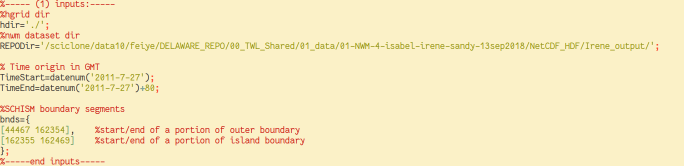
The NWM dataset dir should contain netcdf files with names like "201107010000.CHRTOUT_DOMAIN1.nc", which can be downloaded following the instructions for " NWM reanalysis databases". Note that the 4 nodes (defining the SCHISM boundary to be coupled) mentioned in the previous section are specified in the inputs.
Run the script and check the two diagnostic plots. The first one highlights the portion of the SCHISM boundary used for coupling: 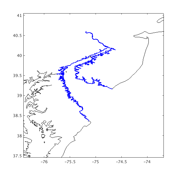The second one illustrates the magnitudes of point sources (time-averaged) by circles of different sizes: In this case, the largest source inside the Delaware Bay is flowing into the Delaware River and the second largest is into the Schuylkill River. A constant discharge is imposed at the head of Susquehanna River.

The following files will be generated under the current directory:

source_sink.in: element IDs where sources and sinks are imposed.
vsource.th: time (seconds; first column) history of flow rate (m³/s; the 2nd to the last columns) at each source (inflow) element.
msource.th: time (seconds; first column) history of tracer concentrations at each source element.
vsink.th: time (seconds; first column) history of flow rate (m³/s; the 2nd to the last columns) at each sink (outflow) element.

Put them under your run directory.

■